First look at RAM utilization

mathuin · 20 June 2022 01:20

This is the first of I hope many runs where I attempt to determine the RAM consumption of different stages under different conditions.

I have Docker Desktop running with 8 CPUs and 56G of RAM on my Mac M1 Max laptop. I have configured a one-node Kubernetes cluster which has Prometheus and Grafana installed within it. I ran a single job and monitored its RAM utilization, making annotations for the ending of the stages that looked relevant. The job had 296 images (average size about 8.5MB) and had the following command line: --rerun-all --pc-quality high --min-num-features 15000 --feature-quality high --pc-filter 0 --auto-boundary.

The annotations from left to right:

16:57:26 end of opensfm detect_features, beginning of opensfm match_features
17:01:57 end of opensfm match_features, beginning of opensfm reconstruct
17:15:28 end of opensfm reconstruct, beginning of opensfm undistortion
17:20:26 end of opensfm, beginning of openmvs densifypointcloud
17:36:18 end of estimated depth maths, beginning of fused depth maps
17:39:00 end of fused depth maps, beginning meshing
17:48:29 end of meshing, beginning of texturing
17:52:43 end of texturing, beginning of georeferencing

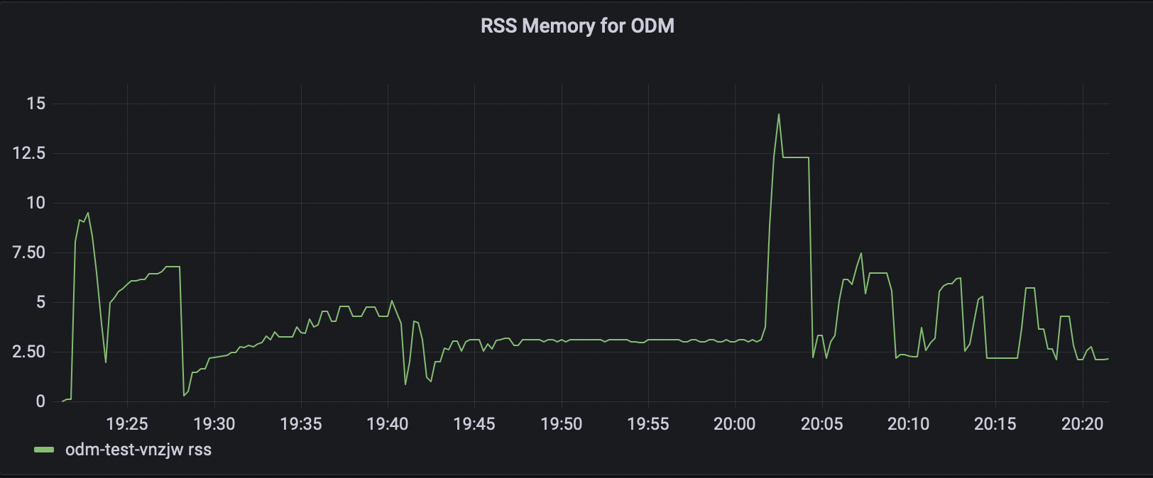
The two stages that used the most memory were opensfm detect_features which peaked at about 9.3G and fused depth maps which went to 15G and stayed there for about two minutes.

The next stuff on my short list: add DTM and DSM, see what happens when either or both qualities are set to ultra, process half the images to see how the curves change.

mathuin · 20 June 2022 20:28

The addition of DSM and DTM (and Euclidean map) is the reason for the extra bumps at the end.

The addition of --pc-tile didn’t have the impact I had hoped it would.

Next up: ultra for each of feature and point cloud – and if those blow up, I’ll try medium for comparison’s sake.

mathuin · 21 June 2022 05:16

This is with features set to ultra. Note the RAM bumps up to three times the original value. It takes longer to process the features, but that’s the RAM impact.

This is with pc set to ultra. Now the tiling is more effective, keeping the max RAM utilization below 25G for the most part.

Next step: ultra for both pc and features!

Saijin_Naib · 21 June 2022 11:20

Wonderful stuff! If you test binary features you’ll see that they use a small fraction of what SIFT and HAHOG do.

mathuin · 21 June 2022 14:38

This is ultra for both pc and features. This whole run fit in 32G – ultra doubled the point cloud requirements but the feature requirements went up by a factor of five!

Next up: the impact on the number of images. This data was collected with three flights within about an hour – I will separate out one flight and run that, then the other two flights, to give me three data points.

mathuin · 21 June 2022 14:42

Interesting! Where can I learn more about the pros and cons of each feature type?

Saijin_Naib · 21 June 2022 15:14

I’m working on a meta-analysis for the docs update, but I can send you a dump of PDFs (unsorted, no notes currently) if you’d like to read what I’ve been reading.

TLDR is SIFT currently gives us the best matching 95% of the time, with HAHOG sometimes outperforming it at a time cost.

AKAZE is supposed to handle small images well compared to other methods, but our implementation of AKAZE limits it.

ORB, according to OpenCV authors who created it, should outperform or match SIFT when properly tuned for a great time/resource savings. Our implementation limits it.

What I’ve found is that for high-quality data, ORB with ultra can be used to keep resource consumption significantly lower than SIFT on the same dataset.

For example, a dataset that used 32GB RAM + 60GB SWAP under SIFT (ultra, 15k features) used about 8GB RAM under ORB (ultra, 15k features).

mathuin · 22 June 2022 07:23

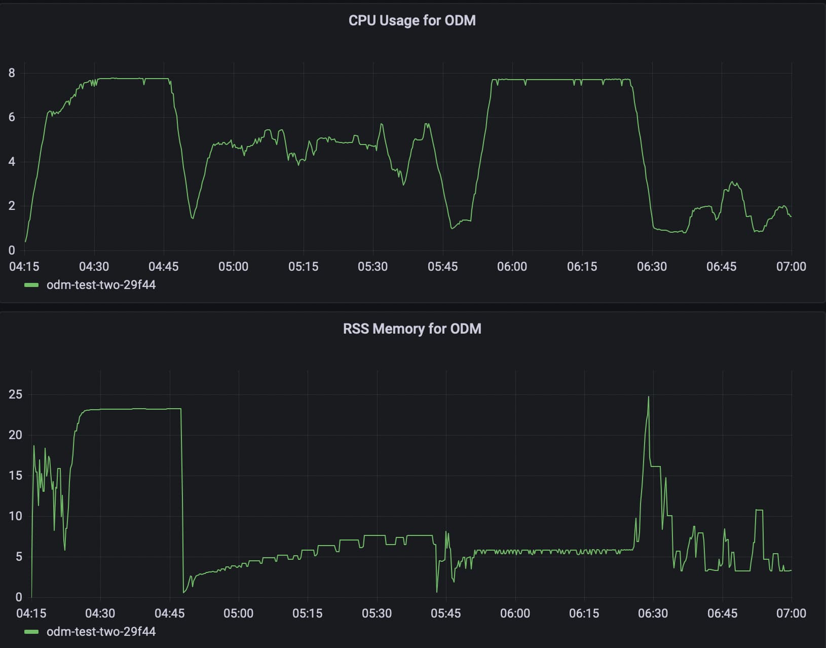
Today we have CPU graphs as well! The CPU tops out during opensfm match_features and densifypointcloud, which isn’t where I had expected.

Anyway, this is the first flight with 114 images (-90 degree camera angle, 0 degree grid rotation if it matters), so roughly one-third of the original dataset. All the settings are the same as the previous run – ultra/ultra with PC tiling. The max RAM used during opensfm is 15.4G, or half the full run, and it’s flat. Weird. Anyway, the point cloud spikes are pretty much the same as before, though only to 22.3G.

This is the other two flights with 182 images (-85 degree camera angle, 60 and 80 degree grid rotation), and I am surprised to see how long it took to do opensfm reconstruct and the densifypointcloud/depth math stuff. Only the latter appears to have been CPU-bound.

I am getting a little closer to my goal of a resource model based on number of images. I haven’t done the math or anything, but for this config, it looks like 2G RAM per CPU per 100 images might work. I think. I don’t know, it’s late, I’ll look at this more tomorrow.

mathuin · 25 June 2022 00:14

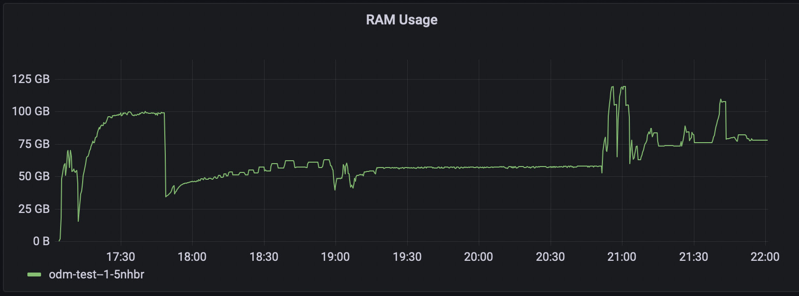
I made one last run today but this time I used my Kubernetes cluster. I used a g-16vcpu-64gb node which costs about $1.50/hr just to see what would happen. I used all the images, ultra for features and point cloud, and point cloud tiling. I left CPU unconstrained, but limited the memory to 57 gibibytes – or so I thought…

Well, it certainly used up all the CPUs, but not at the same spots. Hmm! It also took like four hours. Sigh, so much for faster.

The previous graphs for memory were showing resident set size, which wasn’t what I thought it was after all. This is a common thing to get wrong – there’s probably half a dozen Medium posts and a bunch of StackOverflow answers on the topic – so when I set up monitoring on my cluster I used working set as it’s the one that if exceeded will cause the job to be OOMkilled. Except … the job oversaturated the memory limits by almost 200%. Clearly I have not yet gotten it right.